Jenny Wagner, PhD, MPH
Department of Public Health
California State University, Sacramento

Introduction

Probability distributions are a fundamental concept in statistics and public health research. They describe how the values of a random variable are distributed, information which gives us a mathematical framework to quantify uncertainty and make predictions about data. In simpler terms, a probability distribution shows the likelihood of different outcomes for a given variable. In the real world, they are used to describe patterns in health-related data - for example, the distribution of disease incidence, patient wait times, or the effectiveness of interventions.

There are two main types of probability distributions, discrete and continuous probability distributions, discussed below.

Discrete Probability Distributions

Discrete probability distributions are used for variables that can take on a finite or countable number of distinct values (i.e., for discrete random variables). Each value has a specific probability associated with it. For example, the number of new cases of a disease reported in a week is a discrete variable, as it represents a count (e.g., 0, 1, 2, …). We will focus on two commonly used discrete probability distributions:

Binomial Distribution: Models the probability of a specific number of “successes” in a fixed number of independent trials, where each trial has the same probability of success. For example, we might use the binomial distribution to estimate the probability of a certain number of patients recovering after a new treatment or to predict the proportion of smokers in a sample of adults.
Poisson Distribution: Models the probability of a given number of events occurring in a fixed interval of time and space, assuming the events happen independently and at a constant average rate. For example, we might use the Poisson distribution to model the number of emergency room visits in a day or estimate the number of disease outbreaks in a year in a specific region.

Continuous Probability Distributions

Continuous probability distributions are used for variables that can take on an infinite number of values within a given range (i.e., for continuous random variables). Probabilities are represented as areas under a curve, as the probability of any single exact value is effectively zero (because, again, these variables can take on an infinite number of values). For example, body mass index (BMI) is a continuous variable, as it can take on any value within a realistic range (e.g., 18.5, 24.7). The most commonly used continuous probability distribution is the Normal distribution, which is widely used to model data in public health and is considered the most important probability distribution in statistics.

Normal Distribution: A continuous probability distribution characterized by a symmetric, bell-shaped curve. It is defined by its mean, which determines the center of the distribution, and standard deviation, which determines its spread. The normal distribution is often used to analyze continuous health metrics (e.g., BMI, cholesterol levels, blood pressure, etc.) and serves as the foundation for many statistical methods, including confidence interval estimation and hypothesis testing.

A solid understanding of probability distributions will be important a we move toward statistical methods like estimation and hypothesis testing in the coming weeks.

Objectives

After completing Lab 3, you will be able to:

Construct and interpret a discrete probability distribution.
Calculate probabilities using discrete and continuous probability distributions for public health scenarios.
Calculate measures of center and spread for discrete probability distributions.
Visualize discrete and continuous probability distributions.

Tasks

Lab 3 is divided into two parts. Part 1 focuses on discrete probability distributions based on real data, like the example discussed in this week’s lecture video. For Part 1 you will use the dataset called “substances.csv” which you can download from Canvas. Part 2 focuses on theoretical probability distributions - specifically, the Binomial, Poisson, and Normal distributions. For Part 2 you will not need any data files. Rather, we will apply R functions that already contain information about these theoretical distributions to given public health scenarios.

When you are ready to start Lab 3:

First create a new R Markdown file using the instructions on the Assignment Guidelines page. Save this .Rmd file in a folder dedicated to Lab 3 materials.
Next, download and save the dataset called “substances.csv” in the same folder as your Lab 3 R Markdown file.
Finally, proceed to read through and carry out each of the tasks detailed below. As usual, you will begin by loading R packages, setting your working directory, and importing the dataset.

Part 1: Discrete Probability Distributions Based on Real Data

Part 1 is based on the following scenario: Suppose patients who were involved in a problem gambling treatment program were surveyed about co-occurring drug and alcohol addictions. Let the discrete random variable ‘X’ represent the number of co-occurring addictive substances used by the subjects. The dataset labeled “substances.csv” contains two variables:

A study ID number corresponding to each individual patient.
The number of substances used by the corresponding patient.

1. Install and load R packages

In this Lab we will continue to work with functions contained within the ‘tidyverse’ package. We will also use functions from the ‘stats’ package, which may be new for you. If you have not previously installed this package, copy and paste the following into your Console (bottom-left window), then click Enter or Return to execute the code:

install.packages("stats")

Once you have installed the new package, load the required packages using the library() function as follows:

# load packages
library(tidyverse)
library(stats)

2. Set your working directory

Set your working directory using the setwd() function (see Assignment Guidelines for detailed instructions).

setwd("YOUR FILE PATH HERE")

3. Import the dataset into RStudio

Use the read.csv() function to import the “substances.csv” data file. Remember that this file must be saved in the working directory you specified in the above step.

# import dataset
data <- read.csv("substances.csv") %>% select(-X)

Note: Sometimes when importing a CSV file into RStudio, a column called ‘X’ is added to the dataset to identify the observation number. My personal preference is to drop this column, which is what the %>% select(-X) part of the code above is doing. If you ever notice that an ‘X’ column is added to your dataset, you can use the same code to remove it. But again, this is a personal preference. We could choose leave the ‘X’ column in the dataset if we wanted to; it’s not hurting anything.

After running the above code chunk, you should see an object called data in your Environment window with 777 observations and 2 variables (defined above).

4. Construct a discrete probability distribution

To construct a discrete probability distribution for the number of co-occurring substance addictions, we first need to create a table showing the frequency and relative frequency for this discrete distribution as follows:

# construct frequency table and save it as a new dataframe
subs <- as.data.frame(table(data$substances))

A brief breakdown of this code:

table(data$substances): Creates a frequency table of the substances variable in the data dataset. The table counts the occurrences of each unique value in the substances variable, producing a summary of how often each substance appears.
as.data.frame(): Stores the frequency table as an object in our Environment with two columns: one column for the unique values in substances and another column for their respective counts.
subs <- ...: Names the resulting object subs. The subs object will now contain two columns where:
- The first column (generically called Var1) holds the unique values of the substances variable.
- The second column (Freq) holds the corresponding frequencies (counts) of those values.

Let’s click on the subs object in our Environment to see what it looks like. We can also use the print() command as follows to show the table in the Console (bottom-left) window:

# print frequency table
print(subs)

##    Var1 Freq
## 1     0  144
## 2     1  342
## 3     2  142
## 4     3   72
## 5     4   39
## 6     5   20
## 7     6    6
## 8     7    9
## 9     8    2
## 10    9    1

As expected, we see two variables, Var1 (the number of co-occurring substances) and Freq (the number of people in our dataset with each correponding number of co-occurring substances).

When constructing a discrete probability distribution, the goal is to represent the likelihood of each category or value in the dataset. To do this, we need to calculate relative frequencies, which represent the proportion of occurrences for each category relative to the total number of observations. For our scenario here, this means calculating the relative frequency of each number of co-occurring substances by dividing the frequency in each category by the total number of observations. We can create a new variable for the relative frequencies in our subs object as follows:

# create a new variable for the relative frequency 
    # relative frequency = the proportion of subjects with each number of substances used
subs <- subs %>% mutate(rel_freq = Freq/(sum(Freq)))

This line of code creates a new variable called rel_freq using the frequencies generated previously. A more detailed explanation:

subs: This is the data frame being modified. It contains a frequency table where one column (Freq) holds the counts for each category.
subs %>%: Passes the subs object, which contains the frequency table, through the mutate function. Remember, the pipe operator (we’ve seen this several times now!) is like saying “and then”. We are telling R, “use the data in the object subs and then create a new variable with the mutate() function.”
mutate(): A function used to create new variables or modify existing ones in a data frame. In this case, it adds a new column called rel_freq to the subs data frame.
rel_freq = Freq / (sum(Freq)):
- Freq: Refers to the column in subs that holds the raw frequencies (counts) of each category.
- sum(Freq): Calculates the total frequency (i.e., the sum of all counts in the Freq column).
- Freq / (sum(Freq)): Divides each frequency value by the total frequency to compute the relative frequency for each category. This gives the proportion of the total observations that fall into each category.
subs <-: Reassigns the modified data frame back to the subs object, updating it with the new rel_freq column.

Let’s again use the print() command to view the updated table as follows:

# print frequency table
print(subs)

##    Var1 Freq    rel_freq
## 1     0  144 0.185328185
## 2     1  342 0.440154440
## 3     2  142 0.182754183
## 4     3   72 0.092664093
## 5     4   39 0.050193050
## 6     5   20 0.025740026
## 7     6    6 0.007722008
## 8     7    9 0.011583012
## 9     8    2 0.002574003
## 10    9    1 0.001287001

As expected, we see a new variable, rel_freq, which tells us the relative frequency (or proportion) of the sample with each corresponding number of co-occurring substance addictions.

Next, let’s visualize this probability distribution using the barplot function:

# generate a simple bar chart for sex
barplot(subs$rel_freq, 
        xlab = "Number of co-occurring substance addictions", 
        ylab = "Relative frequency", 
        col = "gray",
        names.arg = subs$Var1)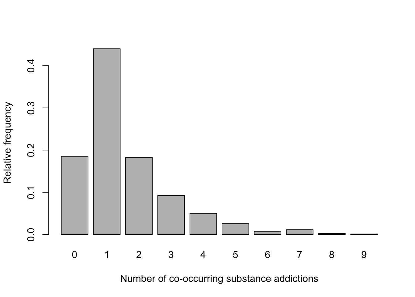

Visualizing the probability distribution in this way allows us to quickly see the most and least likely outcomes.

5. Calculate probabilities from a discrete probability distribution

When we created the subs object, the discrete random variable ‘X’ (currently labeled Var1) defaulted to a factor variable. In previous Labs we have converted numeric variables to factors. Here, however, it will be helpful to convert Var1 from a factor variable to a numeric variable, since we know the values represent quantities - the number of co-occurring substance addictions - not categories. Converting Var1 to a numeric variable will ensure it is treated appropriately in our analyses.

We need to use a two-step process to convert a factor variable to a numeric variable. We first need to convert the factor variable to a “character” variable - basically, text - using the as.character() function, then to a numeric variable using the as.numeric() function. Very strange, I know. If we do not first convert to a character variable, R will drop the category corresponding to zero co-occurring substances, and we don’t want that to happen.

# convert factor to numeric variable
subs$Var1 <- as.character(subs$Var1) # first convert to character 
subs$Var1 <- as.numeric(subs$Var1)

Now that we have formatted our variables appropriately, we can calculate probabilities for specified numbers of co-occurring substance addictions. For example, suppose we want to know the probability that an individual selected at random uses exactly five addictive substances. For a specific number of co-occurring substances (in this case, 5), we can find this answer by looking directly at our discrete probability distribution. When we look at the row where Var1 is equal to 5, we see that rel_freq is equal to 0.025740026. This means that the probability a randomly selected person from the sample has 5 co-occurring substance addictions is 0.025740026, or about 2.6%.

When we want to know the probability associated with one particular value of our discrete random variable, it is easy enough to use this approach of looking at the table of relative frequencies. However, if we want to know the probability associate with a range of values, the most efficient method is to use code. Let’s walk through a few examples…

a. What is the probability that an individual selected at random used fewer than three addictive substances?

# obtain the probability of fewer than 3 co-occurring substance addictions
subs %>% filter(Var1 < 3) %>% summarise(sum(rel_freq))

##   sum(rel_freq)
## 1     0.8082368

Here, we are taking the sum of relative frequencies where Var1 is less than 3. A brief breakdown of this line of code:

subs %>%: The pipe operator %>% passes the subs object, which contains the probability distributions, to the next function in sequence.
filter(Var1 < 3): Filters the dataset, keeping only the rows where the Var1 column has values less than 3 (i.e., rows where Var1 is equal to 0, 1, or 2 will be retained).
summarise(sum(rel_freq)): The summarise() function creates a summary statistic for the filtered data. By nesting sum(rel_freq) within the summarise() function, we obtain the sum of the rel_freq column (relative frequencies) for the filtered subset.

From the output in our Console window, we find the probability that a randomly selected person from the sample uses fewer than 3 addictive substances is 0.8082368, or about 80.8%.

b. What is the probability that an individual selected at random used more than six addictive substances?

subs %>% filter(Var1 > 6) %>% summarise(sum(rel_freq))

##   sum(rel_freq)
## 1    0.01544402

Here, we are taking the sum of relative frequencies where Var1 is greater than 6. We find the probability that a randomly selected person from the sample uses greater than 6 addictive substances is 0.01544402, or about 1.5%.

Note: In part (a) we filtered for values of Var1 less than 3, while here we are filtering for values of Var1 greater than 6. Otherwise the code is exactly the same.

c. What is the probability that an individual selected at random used between 2 and 5 addictive substances?

subs %>% filter(Var1 >= 2 & Var1 <= 5) %>% summarise(sum(rel_freq))

##   sum(rel_freq)
## 1     0.3513514

This one is a little trickier. Here, we are taking the sum of relative frequencies where Var1 is both greater than or equal to 2 and less than or equal to 5 (in other words, where Var1 is between 2 and 5, inclusive). We find the probability that a randomly selected person from the sample uses between 2 and 5 addictive substances is 0.3513514, or about 35.1%.

6. Calculate measures of center and spread for a discrete probability distribution

Measures of center and spread are useful for summarizing and interpreting a discrete probability distribution. The mean, or expected value, provides the average outcome we would expect if the process were repeated many times. The variance measures how spread out the values are around the mean, which provides insight to the variability or uncertainty in the distribution. The standard deviation, as the square root of the variance, provides a more interpretable measure of spread in the same units as the original variable (in this case, the number of co-occurring substance addictions).

We can use the following to obtain the mean, variance, and standard deviation of this discrete probability distribution:

mean(rep(subs$Var1, subs$Freq)) # mean

## [1] 1.572716

var(rep(subs$Var1, subs$Freq)) # variance

## [1] 2.095543

sd(rep(subs$Var1, subs$Freq)) # standard deviation

## [1] 1.447599

We find the mean number of co-occurring substance addictions is approximately 1.57; this represents the average number of co-occurring addictions we expect across the population at-hand. We find the variance and standard deviation are 2.095543 and 1.447599, respectively. These measures of spread give us a sense of how spread out the values are around the mean and are particularly useful when comparing the spread across different populations.

Part 2: Theoretical Probability Distributions

So far in Lab 3, we’ve explored a discrete probability distribution based on real data by calculating key measures like relative frequencies, the mean, variance, and standard deviation. We can use this concrete example to help us understand how probability distributions are used to summarize and describe patterns in data.

Next, we’ll shift our focus to theoretical probability distributions — specifically, the Binomial, Poisson, and Normal distributions. These distributions are widely used in public health to model and predict outcomes in scenarios where we don’t have all the data but need to make informed decisions. By working with these distributions, we can calculate probabilities for specific events, explore relationships between variables, and gain deeper insight into uncertainty and variability in public health contexts. Let’s see how these tools allow us to answer practical probability questions and ultimately support evidence-based decision-making. We will use a different public health scenario for each probability distribution.

1. Binomial distribution

As discussed in the Introduction section above, the Binomial distribution is used to model the number of successes in a fixed number of independent trials, where each trial has the same probability of “success”. Remember from lecture that the terms “success” and “failure” are arbitrary - a “success” does not necessarily mean a positive outcome. For example, in public health, we are often studying disease outcomes, and “success” might correspond to the occurrence of disease or death.

To calculate probabilities using the Binomial distribution, you need three key values:

n: The number of trials (or sample size).
p: The probability of success in a single trial.
x: The number of successes of interest.

Let’s apply the Binomial distribution to the following scenario…

Suppose, based on data collected by the Centers for Disease Control and Prevention (CDC), an estimate of the percentage of adults who have at some point in their life been told they have hypertension is 48.1% percent. The Binomial distribution can be used if the sample size (n) is less than 10% of the population size (N), i.e., n/N ≤ 0.10. Assume for our scenario that ‘N’ is sufficiently large relative to ‘n’ that the binomial distribution may be used to find the desired probabilities.

Suppose we select a simple random sample of 20 U.S. adults and assume that the probability that each has been diagnosed with hypertension is 0.48. We will use this information to answer each of the probability questions below. For these items, we will use two R functions, dbinom() and pbinom():

dbinom(): This function is used to find the probability for a specific number of successes in a given number of trials. The syntax is dbinom(x, n, p) where x = number of successes, n = number of trials, and p = probability of success.
pbinom(): This function is used to find the cumulative probability up to a specific number of successes. In other words, pbinom() gives us P(X <= x). The syntax is pbinom(x, n, p) where, again, x = number of successes, n = number of trials, and p = probability of success.

a. What is the probability that exactly 8 out of 20 adults in our sample have been diagnosed with hypertension?

In this case, the sample size (n) is 20, the number of successes of interest (x) is 8, and the probability of “success” (i.e., that a person has been diagnosed with hypertension) is 0.48. We can apply the dbinom() function as follows:

# find probability that 8 out of 20 adults will have been diagnosed with hypertension
dbinom(8, 20, 0.48)

## [1] 0.1387513

From the output in the Console window, we find the probability that exactly 8 out of 20 adults will have been diagnosed with hypertension is 0.1387513, or about 13.9%.

b. What is the probability that fewer than 8 out of 20 have been diagnosed with hypertension?

In this case, the sample size (n) is, again, 20, the number of successes of interest (x) is all values less than 8 (i.e., 0 to 7), and the probability of “success” (i.e., that a person has been diagnosed with hypertension) is, again, 0.48. We can apply the pbinom() function as follows:

# find probability that fewer than 8 out of 20 adults will have been diagnosed with hypertension
pbinom(7, 20, 0.48)

## [1] 0.1739206

Remember, the pbinom() function gives us the cumulative probability up to the specified number of successes. So, by specifying x=7, we are telling R to give us the probability of 7 successes, plus the probability of 6 successes, plus the probability of 5 successes, and so on, all the way to 0. In this case, we find the probability of fewer than 8 (i.e., 7 or fewer) out of 20 adults will have been diagnosed with hypertension is equal to 0.1739206, or about 17.4%.

c. What is the probability that 8 or more out of 20 have been diagnosed with hypertension?

Since the pbinom() function will give us the probability that 7 or fewer have been diagnosed with hypertension, as we carried out in part (b) above, we can subtract this probability from 1 to get the probability that 8 or more of the 20 will have been diagnosed with hypertension.

# find probability that 8 or more out of 20 adults will have been diagnosed with hypertension
1 - pbinom(7, 20, 0.48)

## [1] 0.8260794

In this case, we find the probability of 8 or more out of 20 adults will have been diagnosed with hypertension is equal to 0.8260794, or about 82.6%.

d. What is the probability that between 8 and 12 (inclusive) out of 20 have been diagnosed with hypertension?

Finally, to find the probability of a range of successes (e.g., 8 to 12 successes, as in this example) in a binomial distribution, we add together the probabilities for each individual number of successes within that range. Instead of summing them manually, we can use the cumulative probability function pbinom() to make this process easier. Specifically, we calculate the cumulative probability for the upper limit of the range (e.g., P(X≤12)) and subtract the cumulative probability just below the lower limit (e.g., P(X≤7)). This gives the total probability for the range P(8≤X≤12).

# find probability that between 8 and 12 (inclusive) out of 20 adults will have been diagnosed with hypertension
pbinom(12, 20, 0.48) - pbinom(7, 20, 0.48)

## [1] 0.7291661

We find the probability that between 8 and 12 (inclusive) out of 20 adults will have been diagnosed with hypertension is equal to 0.7291661, or about 72.9%.

e. Mean and variance of a Binomial distribution

The mean (μ=n⋅p) of a binomial distribution represents the expected number of successes in a given number of trials, which provides a sense of the central tendency of the distribution. It tells us what we can typically expect to happen if the process is repeated many times. The variance (σ2=n⋅p⋅(1−p)) measures the variability of the distribution, giving us a way to quantify how much the number of successes is likely to deviate from the mean on average. Together, these values help us understand both the average outcome and the spread of possible outcomes.

For our scenario, suppose we want to find the mean and variance of the number of people diagnosed with hypertension in samples of size 20. A straightforward way to do this is to apply the mean and variance formulas shown above, using R as a simple calculator.

# calculate the mean (n*p)  and variance is n*p*(1-p) of the binomial distribution
20*0.48 # mean

## [1] 9.6

20*0.48*(1-0.48) # variance

## [1] 4.992

We find the expected number of people to have been diagnosed with hypertension in a sample of 20 is 9.6, with a variance of 4.992.

f. Visualizing the Binomial distribution

Finally, visualizing the Binomial distribution for a given scenario such as this helps us understand the probability of different outcomes at a glance. It provides a picture of where most of the probability is concentrated, showing the likely range of successes and how extreme outcomes are distributed. We can visualize the Binomial distribution for our scenario (in which the sample size is 20 and probability of success is 0.48) as follows:

# define the range of successes as 0 to 20 for the purposes of our plot
success <- 0:20

# plot the Binomial distribution
plot(success, dbinom(success, size=20, prob=0.48), type = 'h')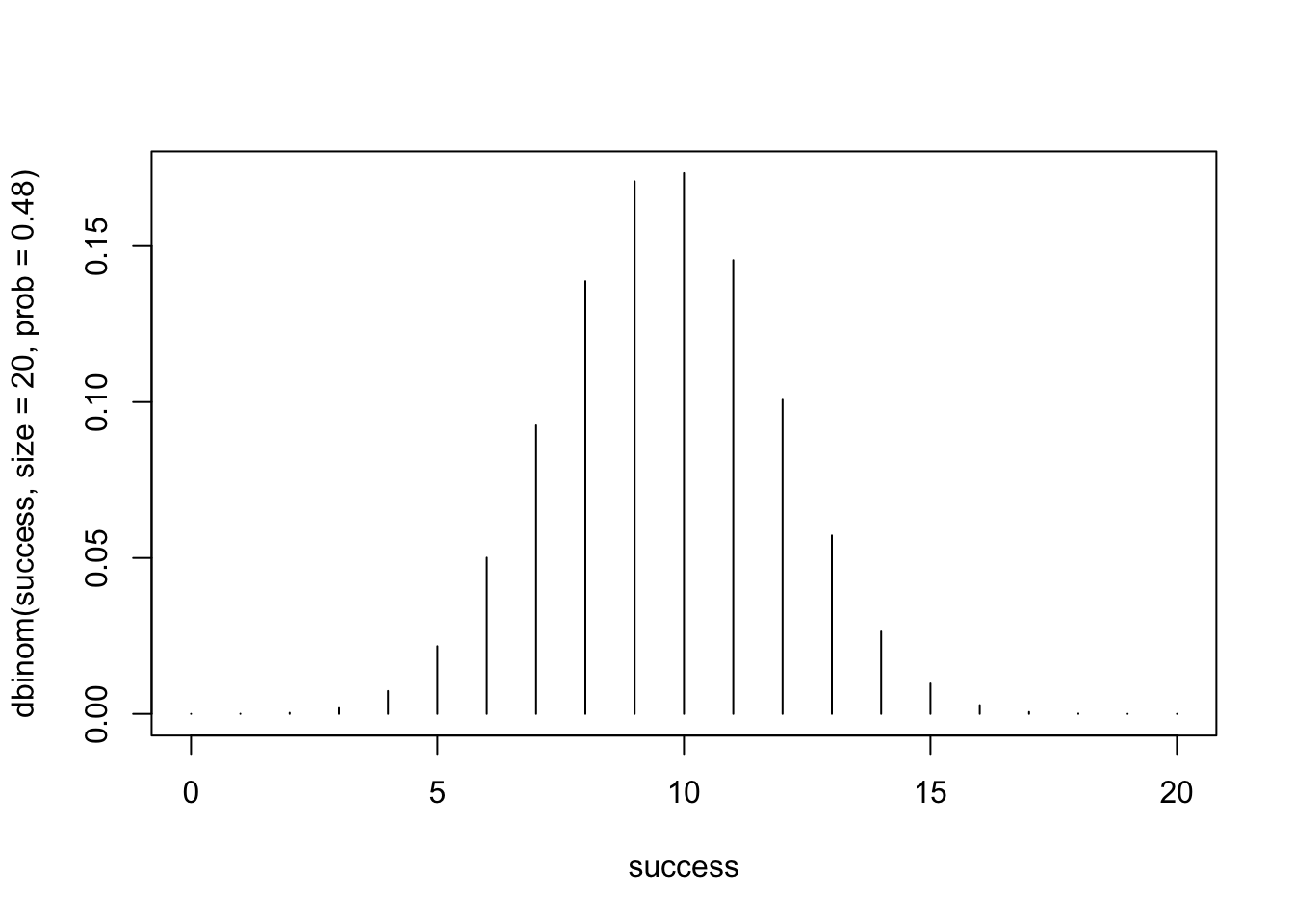

The resulting plot shows the Binomial probability distribution for n=20 trials and a success probability (p) of 0.48. We can interpret this plot as follows:

The x-axis represents the number of successes (X), ranging from 0 to 20. Each tick corresponds to a possible outcome (e.g., 0, 1, 2, … 20 successes).
The y-axis represents the probability of observing each specific number of successes.
Each vertical line corresponds to the probability of a particular number of successes (P(X=x)). The height of the line shows how likely that number of successes is.
The distribution is bell-shaped, with the highest probability (peak) near the expected number of successes, which we found previously was 9.6. Since we can’t actually have 9.6 successes (since ‘X’ is discrete), we see the highest probabilities (i.e., the most likely outcomes) correspond to values 9 and 10.
Finally, the probabilities taper off as you move toward 0 or 20 successes, where extreme outcomes are less likely.

2. Poisson distribution

As discussed previously, the Poisson distribution models the number of events occurring in a fixed interval of time and space, assuming the events occur independently and at a constant average rate. To use the Poisson distribution, you need:

λ (lambda): The average number of events in the interval.
x: The number of events of interest.

Let’s apply the Poisson distribution to the following scenario…

In a certain population, an average of 13 new cases of esophageal cancer are diagnosed each year. Suppose the annual incidence of esophageal cancer follows a Poisson distribution. We will use this information to answer each of the probability questions below. For these items, we will use two R functions, dpois() and ppois():

dpois(): This function is used to find the probability that exactly ‘x’ number of events occur within the time period. The syntax is dpois(x, λ), where ‘x’ is the number of events of interest, and ‘λ’ is the mean.
ppois(): This function gives the cumulative probability that ‘x’ or fewer events occur within the time period. The syntax is ppois(x, λ), where, again, ‘x’ is the number of events of interest, and lambda is the mean.

a. What is the probability that, in a given year, the number of newly diagnosed cases of esophageal cancer will be exactly 10?

# find probability that exactly 10 cases of esophageal cancer will be diagnosed
dpois(10, 13)

## [1] 0.08587015

From the output in the Console, we find that, when the mean incidence is 13 cases annually, the probability that exactly 10 cases of esophageal cancer are diagnosed in a given year is 0.08587015, or about 8.6%.

b. What is the probability that, in a given year, the number of newly diagnosed cases of esophageal cancer will be 12 or fewer?

# find probability that 12 or fewer cases of esophageal cancer will be diagnosed
ppois(12, 13)

## [1] 0.4631047

We find that, when the mean incidence is 13 cases annually, the probability that 12 or fewer cases of esophageal cancer are diagnosed in a given year is 0.4631047, or about 46.3%.

c. What is the probability that, in a given year, the number of newly diagnosed cases of esophageal cancer will be at least eight?

# find probability that 8 or more cases of esophageal cancer will be diagnosed
1 - ppois(7, 13)

## [1] 0.9459718

We find that, when the mean incidence is 13 cases annually, the probability that 8 or more cases of esophageal cancer are diagnosed in a given year is 0.9459718, or about 94.6%.

d. What is the probability that, in a given year, the number of newly diagnosed cases of esophageal cancer will be between nine and 15 (inclusive)?

# find probability that between 9 and 15 (inclusive) cases of esophageal cancer will be diagnosed
ppois(15, 13) - ppois(8, 13)

## [1] 0.663849

We find that, when the mean incidence is 13 cases annually, the probability that between 9 and 15 (inclusive) cases of esophageal cancer are diagnosed in a given year is 0.663849, or about 66.4%.

e. Create a plot to visualize this Poisson distribution.

As with our plot of the Binomial distribution above, plotting the Poisson distribution can help us understand where the highest probabilities are concentrated. In other words, the plot can give us a quick idea of the most likely outcomes. We can visualize the Poisson distribution for our scenario (in which the mean number of events is 13) as follows:

events <- 0:30
plot(events, dpois(events, lambda = 13), type = 'h')

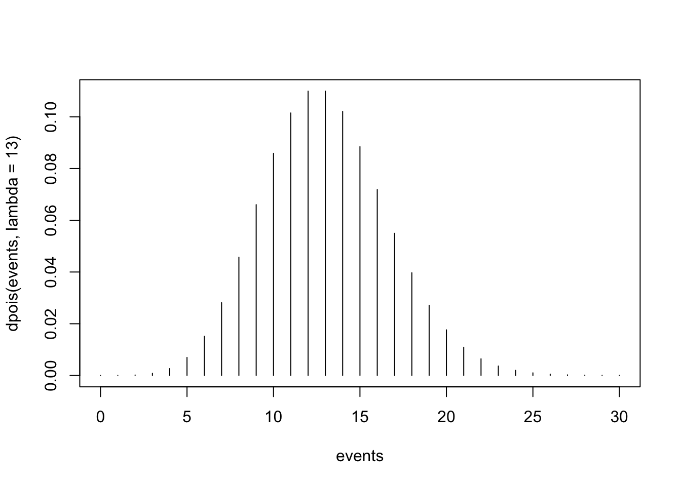
The resulting plot shows the Poisson probability distribution for the number of events (X) ranging from 0 to 30, with an average rate (λ) of 13. Here’s how to interpret the plot:

The x-axis represents the possible number of events (X), ranging from 0 to 30. Each tick corresponds to a specific count of events (e.g., 0, 1, 2, …, 30). Note that 30 here is arbitrary - this number of events simply allowed for the bulk of the distribution to be visible on the plot (since the probabilities are very tiny after about 25 events).
The y-axis represents the probability of observing a specific number of events. Each vertical line corresponds to the probability of observing exactly that many events (P(X=x)). The height of the line shows the likelihood of that particular outcome.
The plot will peak near λ=13, which is the average number of events, reflecting that this outcome is most likely.
The probabilities taper off to the left (fewer events) and the right (more events) of the mean. The distribution is right-skewed, which is characteristic of the Poisson distribution (because, technically, there is some probability associated with any number of events), particularly when λ is not very large.

3. Normal distribution

Finally, the Normal distribution is a continuous probability distribution often used to model data that are symmetrically distributed around a mean. To calculate probabilities using the Normal distribution, you need:

μ (mu): The mean of the distribution.
σ (sigma): The standard deviation of the distribution.
x: The value or range of values for which you want to calculate the probability.

For example, the Normal distribution can be used to estimate the likelihood of an individual’s BMI falling within a specific range in a population. By specifying the population mean BMI (μ), the standard deviation (σ), and the range of interest (x), you can determine the probability of the outcome.

Remember, unlike the Binomial and Poisson distributions, which are discrete, the Normal distribution is continuous. This means that probabilities are not associated with specific values of X but rather with ranges of values. Since the Normal distribution has an infinite number of possible values within any interval, the probability of any single exact value of X is essentially zero. Instead, we calculate probabilities for a range of values by finding the area under the standard normal curve between two points.

Let’s apply the Normal distribution to the following scenario…

One of the variables collected in Birth Registry data is pounds gained during pregnancy. According to data from the entire registry for 2021, the number of pounds gained during pregnancy was approximately normally distributed with a mean of 30.23 pounds and a standard deviation of 13.84 pounds. We will use this information to answer each of the probability questions below. For these items, we will need only one R function, pnorm():

pnorm(): This function gives the cumulative probability that a random variable ‘X’ takes a value less than or equal to ‘x’. The syntax is pnorm(x, mean, sd).

a. Find the probability that a randomly selected mother in 2021 gained less than 15 pounds during pregnancy.

# find probability that a randomly selected mother gained less than 15 pounds
pnorm(15, 30.23, 13.84)

## [1] 0.1355716

From the output in the Console, we find the probability that a randomly selected mother in 2021 gained less than 15 pounds during pregnancy is 0.1355716, or about 13.6%.

b. Find the probability that a randomly selected mother in 2021 gained more than 40 pounds during pregnancy.

# find probability that a randomly selected mother gained more than 40 pounds
1 - pnorm(40, 30.23, 13.84)

## [1] 0.2401174

We find the probability that a randomly selected mother in 2021 gained more than 40 pounds during pregnancy is 0.2401174, or about 24.0%.

c. Find the probability that a randomly selected mother in 2021 gained between 15 and 40 pounds during pregnancy.

# find probability that a randomly selected mother gained between 15 and 40 pounds
pnorm(40, 30.23, 13.84) - pnorm(15, 30.23, 13.84)

## [1] 0.6243109

We find the probability that a randomly selected mother in 2021 gained between 15 and 40 pounds during pregnancy is 0.6243109, or about 62.4%.

d. Create a plot to visualize this Normal distribution.

Visualizing the Normal distribution associated with a given scenario can help us understand the distribution of values and predict probabilities for ranges of interest. We can visualize the Normal distribution for our scenario as follows:

curve(dnorm(x, 30.23, 13.84), from=0, to=60)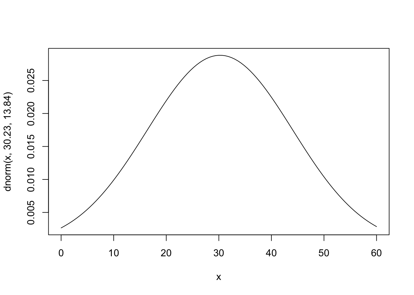

The plot shows the Normal distribution with a mean (μ) of 30.23 and a standard deviation (σ) of 13.84. Here’s how to interpret the plot:

The x-axis represents the range of possible values for the variable of interest, spanning from 0 to 60 (an arbitrary range, but one that allows us to view essentially the whole distribution).
The y-axis represents the probability density for the corresponding x-values. The height of the curve at a given x-value indicates how densely the data are distributed around that value but does not represent the actual probability of a single point (since this is a continuous distribution).
The curve is bell-shaped and symmetric, with the peak occurring at μ=30.23, which is the most likely value.
Most of the probability is concentrated within 1-2 standard deviations of the mean (approximately 30.23 ± 13.84). The tails taper off gradually, meaning that values far from the mean (e.g., below 10 or above 50) are less likely but still possible.

Summary

In Lab 3, we explored theoretical probability distributions, including the Binomial, Poisson, and Normal distributions. Probability distributions are essential in public health for modeling uncertainty, estimating disease risk, and predicting health outcomes in populations. They help us understand the likelihood of events such as the spread of infectious diseases, the probability of treatment success, or the expected number of emergency room visits. While these concepts may feel abstract, they provide the foundation for everything we do in statistical inference — like helping us estimate population parameters, assess variability, and determine the likelihood of different outcomes. While we won’t focus heavily on probability theory in this course, this foundational knowledge will be important as we move into statistical inference, including confidence interval estimation, hypothesis testing, and regression analysis.

When you are ready, please submit the following to the Lab 3 assignment page on Canvas:

An R Markdown document, which has a .Rmd extension
A knitted .html file

Please reach out to me at jenny.wagner@csus.edu if you have any questions. See you in class!

Lab 3: Probability Distributions