Lab 8: Logistic Regression
Introduction
In Lab 8, we’ll shift our focus to a new type of model: logistic regression. Last week, we discussed how linear regression is useful for modeling continuous outcomes. Logistic regression is used when the outcome is binary — that is, when there are only two possible values. In public health research, this often means modeling the presence or absence of a health outcome, such as disease status or event occurrence.
We’ll use the Framingham Heart Study dataset to investigate how baseline characteristics like age, sex assigned at birth, smoking status, BMI, blood pressure, cholesterol, and diabetes diagnosis relate to the risk of having a heart attack during the study’s follow-up period. Our outcome of interest here is binary: whether or not a participant experienced a heart attack during the follow-up period (yes/no).
Like linear regression, logistic regression allows us to examine associations between predictors and an outcome, but instead of estimating the mean of a continuous outcome, it models the probability of a binary outcome. Because probabilities must fall between 0 and 1, logistic regression uses the logit function (the log of the odds) to transform probabilities into a continuous scale that can be modeled using a linear equation.
There are several important assumptions to keep in mind when using logistic regression:
- The outcome variable is binary.
- Observations are independent of one another.
- There is a linear relationship between the predictor of interest and the log odds of the outcome.
- There is no problematic multicollinearity among predictors.
- The sample size is sufficiently large for stable estimates
- A general rule of thumb is that there should be at least 10 cases of the less frequent category of the outcome per predictor variable. For example, if you plan to use 7 predictor variables in a logistic regression model, you should have at least 70 cases of the less frequent category of your outcome of interest.
Objectives
After completing Lab 8, you will be able to:
- Fit a logistic regression model using R/RStudio.
- Check assumptions of logistic regression.
- Exponentiate regression coefficients to obtain odds ratios.
- Interpret odds ratios.
Tasks
For Lab 8, we will continue our exploration of risk factors for
cardiovascular disease using the Framingham Heart Study. In this Lab we
will focus on a specific outcome: the occurrence of heart attacks during
the follow-up period (called MI_FCHD). Our goal is to build
a logistic regression model using baseline characteristics collected at
the start of the study to identify significant predictors of heart
attack risk.
When you are ready to start Lab 8:
- First create a new R Markdown file using the instructions on the
Assignment Guidelines page. Save this
.Rmdfile in a folder dedicated to Lab 8 materials. - Next, download the file called “frmgham2.csv” from Canvas and save it in the same folder as your Lab 8 R Markdown file. Note that this is the original Framingham Heart Study dataset, which we have used in prior Labs.
- Finally, proceed to read through and carry out each of the tasks detailed below. As usual, you will begin by loading R packages, setting your working directory, and importing the dataset.
1. Install and load R packages
We will use the following packages in this Lab:
# load packages
library(tidyverse)
library(naniar)
library(stats)
library(lmtest)
library(performance)
2. Set your working directory
Set your working directory using the setwd() function
(see Assignment Guidelines for detailed instructions).
setwd("YOUR FILE PATH HERE")3. Import the dataset into RStudio
Use the read.csv() function to import the “frmgham2.csv”
dataset. For this to work, this file will need to be saved in the
working directory you specified in the above step.
4. Prepare the dataset for analysis
As we are starting here with the original Framingham Heart Study dataset (and not the cleaned version we have used in a few prior Labs), we will need to follow a few steps to prepare the dataset for analysis. First, we will filter the dataset to contain only the baseline sample. This is because we are going to investigate the association between baseline characteristics and heart attack risk.
Note: Although we will be analyzing only the baseline observations, our outcome of interest — whether a participant experienced a heart attack (recorded in the dataset as
MI_FCHD) applies to the entire follow-up period. This variable is binary, where “1” indicates that a participant experienced a heart attack at some point during follow-up, and “0” indicates they did not.
In analyzing data from prospective cohort studies such as this, the
standard approach is to start with a disease-free population and observe
the occurrence of new cases over time. As such, we will restrict our
analysis to individuals without prevalent heart disease at baseline. We
can filter the dataset to include only participants without heart
disease at baseline (indicated by the variable PREVCHD) as
follows:
# filter to include only individuals without prevalent heart disease at baseline
data_sub <- data_sub %>% filter(PREVCHD == 0)
Next, let’s retain only the variables we plan to use in our
regression analysis — including our outcome and predictors of interest —
so that our dataset is smaller and more manageable. As discussed above,
we will investigate sex assigned at birth, age, BMI, systolic blood
pressure, total cholesterol level, smoking status, and diabetes status
as possible predictors of heart attack risk. We can retain these
variables using the select() function as follows:
# select variables we want to use in regression analysis
data_reg <- data_sub %>% select(RANDID, SEX, AGE, BMI, SYSBP, TOTCHOL, CURSMOKE, DIABETES, MI_FCHD)
Before we begin our analysis, let’s quickly check for missing data by
nesting the is.na() function within the
colSums() function as follows:
##   RANDID      SEX      AGE      BMI    SYSBP  TOTCHOL CURSMOKE DIABETES
##        0        0        0       19        0       50        0        0
##  MI_FCHD
##        0
From the output, we can see there are 19 missing values for BMI
(BMI) and 50 missing values for total cholesterol
(TOTCHOL). Since there are very few missing values relative
to our sample size, let’s address missingness using complete case
analysis (i.e., remove rows with any missing values), as follows:
Finally, as we have done in prior Labs, let’s identify variables types and modify them as needed:
## 'data.frame':    4172 obs. of  9 variables:
##  $ RANDID  : int  2448 6238 9428 10552 11252 11263 12629 12806 14367 16365 ...
##  $ SEX     : int  1 2 1 2 2 2 2 2 1 1 ...
##  $ AGE     : int  39 46 48 61 46 43 63 45 52 43 ...
##  $ BMI     : num  27 28.7 25.3 28.6 23.1 ...
##  $ SYSBP   : num  106 121 128 150 130 ...
##  $ TOTCHOL : int  195 250 245 225 285 228 205 313 260 225 ...
##  $ CURSMOKE: int  0 0 1 1 1 0 0 1 0 1 ...
##  $ DIABETES: int  0 0 0 0 0 0 0 0 0 0 ...
##  $ MI_FCHD : int  1 0 0 0 0 1 0 0 0 0 ...
Our output contains a list of the variables in our dataset, followed by the variable type, where “num” indicates a variable is a continuous numerical variable and “int” indicates a variable is an integer (i.e., a discrete numerical variable). For our regression analysis, this distinction between continuous numerical variables (“num”) and discrete numerical variables (“int”) will not matter. However, as we have done many times in the past, we should convert any variables that represent categories (rather than quantities) to factor variables. In our dataset, this includes sex assigned at birth, smoking status, diabetes diagnosis, and occurrence of heart attacks during follow-up. We can modify these variables as follows:
# convert sex to unordered factor variable
data_reg$SEX <- factor(data_reg$SEX,
                         levels=c("1", "2"),
                         ordered=FALSE)
# convert smoking status to unordered factor variable
data_reg$CURSMOKE <- factor(data_reg$CURSMOKE,
levels=c("0", "1"),
ordered=FALSE)# convert diabetes status to unordered factor variable
data_reg$DIABETES <- factor(data_reg$DIABETES,
levels=c("0", "1"),
ordered=FALSE)# convert occurrence of heart attack to unordered factor variable
data_reg$MI_FCHD <- factor(data_reg$MI_FCHD,
levels=c("0", "1"),
ordered=FALSE)5. Exploratory data analysis
Before we build our logistic regression model, we should be familiar
with the variables we plan to include. First, we should know the
distribution of our outcome of interest (i.e., we should know how many
people experienced a heart attack during follow-up and how many did
not). We can check the number who experienced a heart attack using the
table() command as follows:
# check how many people in the sample experienced a heart attack during follow-up
table(data_reg$MI_FCHD)
##
## 0 1
## 3577 595From the output, we can see there are 595 participants who experienced a heart attack during follow-up and 3,577 participants who did not.
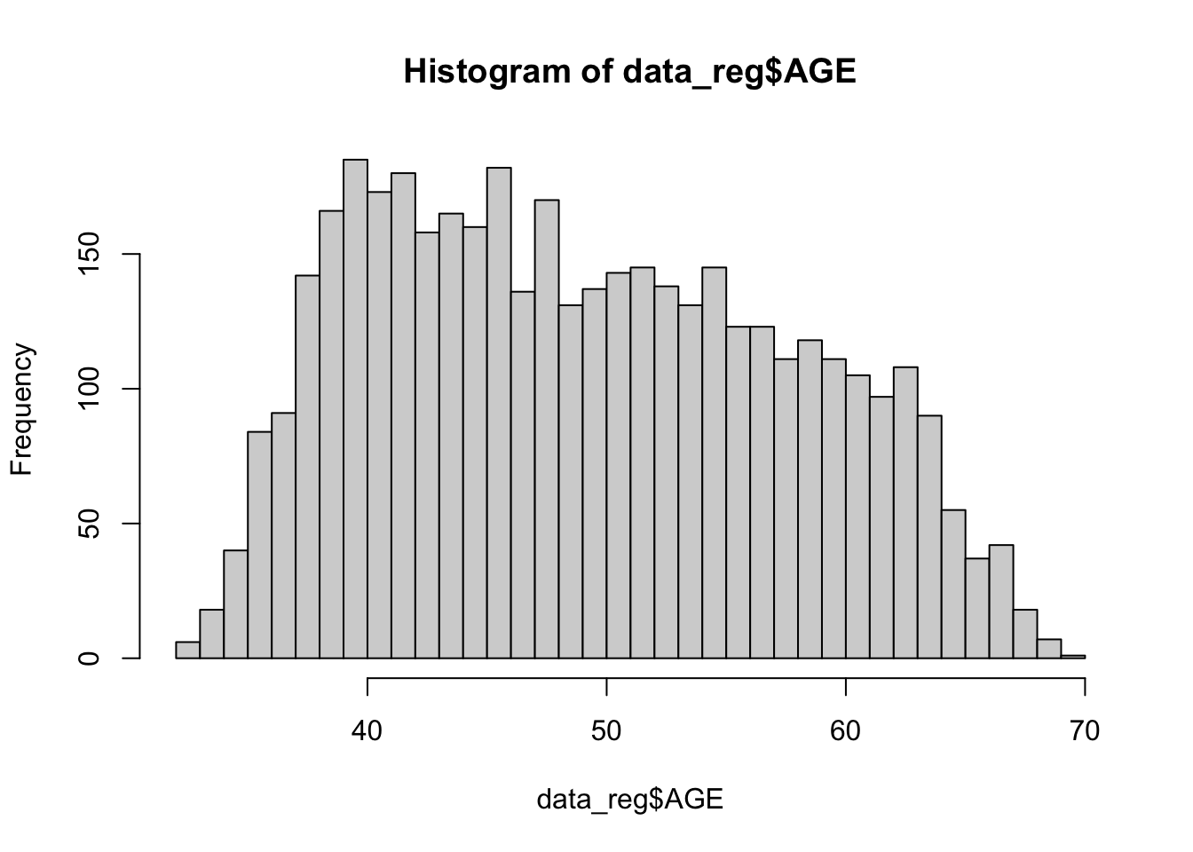
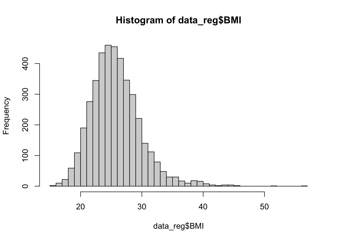
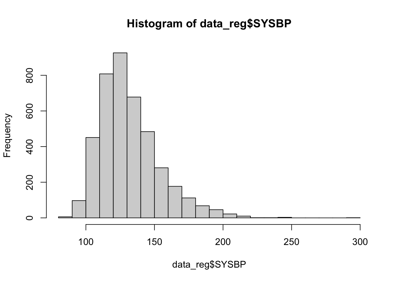
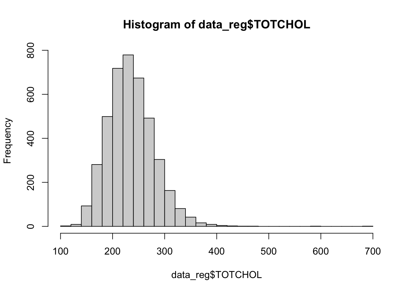
Next, let’s check the distribution of our predictor variables of interest, using histograms for numerical variables and tables for categorical variables, as follows:
##
##    1    2
## 1808 2364##
## 0 1
## 2115 2057##
## 0 1
## 4066 106The histograms above show that BMI, systolic blood pressure, and total cholesterol are right-skewed. While logistic regression does not require numerical predictor variables to be normally distributed, it does assume that each continuous predictor has a linear relationship with the log-odds of the outcome. Skewed predictors may sometimes violate this assumption. As we move forward with modeling, we’ll need to keep in mind whether any variable transformations (e.g., log or square root) might be needed to better meet the linearity of the logit assumption. For now, let’s move on with fitting our initial logistic regression model.
6. Fit logistic regression model
In this step, we will use the glm() function to fit a
logistic regression model. Recall that the goal of logistic regression
is to examine how a set of predictor variables of interest (in this
case, sex at birth, age, BMI, blood pressure, cholesterol, smoking
status, and diabetes) are associated with the probability that a
participant experienced a heart attack during the follow-up period.
We will specify family = binomial because our outcome
variable (MI_FCHD) is binary, meaning it takes the value
“1” if a heart attack occurred and “0” if it did not. The binomial
family tells R to use a logit link function, which models the
log-odds of the outcome as a linear combination of the predictors. In
other words, the model estimates how each predictor affects the log-odds
of having a heart attack, holding the other variables constant. This
allows us to understand the relative contribution of each factor to
heart attack risk while adjusting for the others.
# fit initial logistic regression model
model1 <- glm(MI_FCHD ~ SEX + AGE + BMI + SYSBP + TOTCHOL + CURSMOKE + DIABETES,
              family = binomial, data = data_reg)
Just as we did with linear regression, we can use the
summary() function to view the model results, as
follows:
##
## Call:
## glm(formula = MI_FCHD ~ SEX + AGE + BMI + SYSBP + TOTCHOL + CURSMOKE +
##     DIABETES, family = binomial, data = data_reg)
##
## Coefficients:
##              Estimate Std. Error z value Pr(>|z|)
## (Intercept) -7.559888   0.498172 -15.175  < 2e-16 ***
## SEX2        -1.195035   0.101648 -11.757  < 2e-16 ***
## AGE          0.022749   0.006030   3.773 0.000162 ***
## BMI          0.035429   0.011885   2.981 0.002874 **
## SYSBP        0.015898   0.002203   7.217 5.33e-13 ***
## TOTCHOL      0.007763   0.001059   7.328 2.33e-13 ***
## CURSMOKE1    0.310982   0.099839   3.115 0.001840 **
## DIABETES1    0.905122   0.222462   4.069 4.73e-05 ***
## ---
## Signif. codes:  0 '***' 0.001 '**' 0.01 '*' 0.05 '.' 0.1 ' ' 1
##
## (Dispersion parameter for binomial family taken to be 1)
##
##     Null deviance: 3418.4  on 4171  degrees of freedom
## Residual deviance: 3044.3  on 4164  degrees of freedom
## AIC: 3060.3
##
## Number of Fisher Scoring iterations: 5
The output provides the results of our logistic regression model — which, again, estimates how each predictor is associated with the log-odds of experiencing a heart attack. This may or may not be our “final” model, but for now, let’s get familiar with the output:
- Regression coefficients (labeled “Estimate”)
- Each Estimate represents the change in the log-odds of having a
heart attack for a one-unit increase in that predictor (holding other
variables constant).
- A positive coefficient means that an increase in that predictor increases the log-odds (and therefore the probability) of a heart attack.
- A negative coefficient means that an increase in that predictor decreases the log-odds (and the probability) of a heart attack.
- For categorical variables (like SEX2, CURSMOKE1, and DIABETES1), the coefficient compares the listed category to a reference group (more on this later).
- Each Estimate represents the change in the log-odds of having a
heart attack for a one-unit increase in that predictor (holding other
variables constant).
- Statistical significance
- The Pr(>|z|) column indicates whether the coefficient is statistically significantly different from 0.
- Small p-values (e.g., < 0.05) indicate strong evidence that the predictor is associated with the outcome.
- The asterisks (e.g., *, ) give a quick visual cue of whether a coefficient is significant.
- Model fit metrics
- Null deviance shows how well a model with no predictors (i.e., with only the intercept) fits the data.
- Residual deviance shows the fit of your current model, where a large reduction from null to residual deviance indicates better model fit.
- AIC (Akaike Information Criterion) is another measure of model fit, where lower values indicate better fit when comparing different models.
7. Model diagnostics
Before we interpret and use our model, we first need to run model diagnostics to ensure the assumptions of logistic regression are reasonably met. This means checking: (1) whether each numerical predictor variable has a linear relationship with the log-odds of the outcome, and (2) whether there is any concerning multicollinearity between predictor variables.
Check linearity assumption
We will use the Box-Tidwell Test to check whether each numerical predictor has a linear relationship with the log-odds of the outcome. This test adds an interaction term between each numerical variable and its log-transformed version (e.g., AGE * log(AGE)) to the model. If the relationship between the predictor and the log-odds is truly linear, this interaction term should not be statistically significant. In a nutshell…
- If the interaction term is not significant → the linearity assumption is likely met for that predictor.
- If the interaction term is significant → the relationship is likely nonlinear (in which case we could consider using a variable transformation to try to improve linearity).
When using the Box-Tidwell Test, we should first make sure that all
values for each numerical predictor variable are greater than 0, as the
log of 0 is undefined. To check whether there are any 0 values, you can
open the data_reg object (click on the object in the
Environment window to open it in a new tab), then click on the column
name for each numerical variable to quickly sort the values from lowest
to highest. If you don’t see any 0 values, you can proceed with the
test. If needed, you can add a small constant (e.g., 0.01) to any
variable that has 0 values.
In our case, there are no 0 values for age, BMI, systolic blood pressure, or total cholesterol, so we will continue on to the first step of the test, which is to create new variables for the log of each numerical predictor, which we can do as follows:
# Create new variables for the log of each predictor
data_reg <- data_reg %>% mutate(AGE_log = log(AGE),
                                BMI_log = log(BMI),
                                SYSBP_log = log(SYSBP),
                                TOTCHOL_log = log(TOTCHOL))
Next, we will fit a logistic regression model containing all predictors of interest. This time, however, we will also include interaction terms between each numerical predictor variable and its log version, as follows:
# Fit a model including interactions between variables and their log
bt_model <- glm(MI_FCHD ~ SEX + AGE + I(AGE*AGE_log) +
                          BMI + I(BMI*BMI_log) +
                          SYSBP + I(SYSBP*SYSBP_log) +
                          TOTCHOL + I(TOTCHOL*TOTCHOL_log) +
                          CURSMOKE + DIABETES,
                data = data_reg, family = binomial)
summary(bt_model)
##
## Call:
## glm(formula = MI_FCHD ~ SEX + AGE + I(AGE * AGE_log) + BMI +
## I(BMI * BMI_log) + SYSBP + I(SYSBP * SYSBP_log) + TOTCHOL +
## I(TOTCHOL * TOTCHOL_log) + CURSMOKE + DIABETES, family = binomial,
## data = data_reg)
##
## Coefficients:
## Estimate Std. Error z value Pr(>|z|)
## (Intercept) -14.801311 4.663261 -3.174 0.00150 **
## SEX2 -1.172554 0.103948 -11.280 < 2e-16 ***
## AGE 0.218618 0.336034 0.651 0.51532
## I(AGE * AGE_log) -0.039845 0.068102 -0.585 0.55849
## BMI 0.329809 0.387075 0.852 0.39418
## I(BMI * BMI_log) -0.067996 0.089046 -0.764 0.44510
## SYSBP 0.077129 0.098960 0.779 0.43574
## I(SYSBP * SYSBP_log) -0.010173 0.016467 -0.618 0.53670
## TOTCHOL 0.056288 0.036196 1.555 0.11993
## I(TOTCHOL * TOTCHOL_log) -0.007413 0.005493 -1.349 0.17721
## CURSMOKE1 0.315481 0.100200 3.149 0.00164 **
## DIABETES1 0.933984 0.222574 4.196 2.71e-05 ***
## ---
## Signif. codes: 0 '***' 0.001 '**' 0.01 '*' 0.05 '.' 0.1 ' ' 1
##
## (Dispersion parameter for binomial family taken to be 1)
##
## Null deviance: 3418.4 on 4171 degrees of freedom
## Residual deviance: 3040.9 on 4160 degrees of freedom
## AIC: 3064.9
##
## Number of Fisher Scoring iterations: 5From the model summary, we can see that none of the interaction terms are statistically significant (because p>0.05 in all cases), meaning the linearity assumption is likely met for each numerical predictor, and we won’t need to use any variable transformations. Yay!
Check for multicollinearity
Next, we will check for multicollinearity between predictor
variables. Recall from our discussion of linear regression that
multicollinearity occurs when two or more predictor variables are highly
correlated. This can cause problems in estimating regression
coefficients. Just as we did in Lab 7, we will use the
check_collinearity() function to generate a Variance
Inflation Factor (VIF) for each variable, as follows:
## # Check for Multicollinearity
##
## Low Correlation
##
##      Term  VIF   VIF 95% CI adj. VIF Tolerance Tolerance 95% CI
##       SEX 1.12 [1.09, 1.17]     1.06      0.89     [0.86, 0.92]
##       AGE 1.21 [1.17, 1.26]     1.10      0.83     [0.79, 0.85]
##       BMI 1.13 [1.09, 1.17]     1.06      0.89     [0.85, 0.91]
##     SYSBP 1.28 [1.23, 1.33]     1.13      0.78     [0.75, 0.81]
##   TOTCHOL 1.06 [1.03, 1.10]     1.03      0.95     [0.91, 0.97]
##  CURSMOKE 1.14 [1.11, 1.19]     1.07      0.88     [0.84, 0.90]
##  DIABETES 1.02 [1.01, 1.09]     1.01      0.98     [0.92, 0.99]
From the output, we can see the VIF values (second column from the left) are all close to 1. This means there is no problematic multicollinearity in our original model. Great!
8. Exponentiate regression coefficients
Now that we have verified our original model meets assumptions of
logistic regression, we can proceed with interpreting our results.
Recall that the coefficients from a logistic regression model represent
changes in the log-odds of the outcome for a one-unit increase in each
predictor. While this is useful from a modeling standpoint, log-odds can
be hard to interpret intuitively. To make our results more meaningful,
we can exponentiate the coefficients using the
exp() function. This converts log-odds to odds
ratios, which are easier to interpret and more accessible to a
broader audience. An odds ratio (OR) tells us how the odds of the
outcome change with a one-unit increase in the predictor:
- OR > 1 → increased odds (the predictor is a risk factor for the outcome)
- OR < 1 → decreased odds (the predictor is a protective factor for the outcome)
- OR = 1 → no association (there is no association between the predictor and outcome)
We can exponentiate the regression coefficients from our model by
nesting the coef() function within the exp()
function and save the result to an R object (called
odds_ratios), as follows:
Let’s round the odds ratios to three decimal places and put them in a nice table, as follows:
# put odds ratios in a nice table
odds_ratios <- as.data.frame(round(odds_ratios, 3))
print(odds_ratios)
## round(odds_ratios, 3)
## (Intercept) 0.001
## SEX2 0.303
## AGE 1.023
## BMI 1.036
## SYSBP 1.016
## TOTCHOL 1.008
## CURSMOKE1 1.365
## DIABETES1 2.472In the output, we see two columns - one listing the predictors of interest and the other listing the odds ratio associated with each predictor. In the next section, we’ll discuss how to interpret these results.
9. Interpret odds ratios
If you take away only one thing from this Lab, let it be this: how to correctly interpret an odds ratio. Odds ratios are one of the most commonly reported effect measures in public health research involving binary outcomes. They tell us how the odds of an outcome (like having a heart attack) change in relation to a predictor variable:
- For a continuous variable (like age, BMI, systolic blood pressure,
or total cholesterol), the odds ratio represents the change in the odds
of the outcome associated with a one-unit increase in that variable,
holding all other variables constant.
- To calculate the percent change in odds, we will use the following formula (which should feel very familiar from PUBH 207A): (OR−1) × 100 = % change in odds
- For a categorical variable (like sex assigned at birth, smoking status, or diabetes diagnosis), the odds ratio compares the odds of the outcome for one category relative to a reference category.
For example, we can interpret the odds ratios we obtained in the previous section as follows:
- SEX2 = 0.303 → Participants coded as SEX=2 (females) have 69.7% lower odds of experiencing a heart attack during follow-up compared to males (the reference group, SEX=1), holding all other variables constant.
- AGE = 1.023 → For each additional year of age, the odds of experiencing a heart attack increase by 2.3%, holding all other variables constant.
- BMI = 1.036 → For each one-unit increase in BMI, the odds of having a heart attack increase by 3.6%, holding all other variables constant.
- SYSBP = 1.016 → For each 1 mmHg increase in systolic blood pressure, the odds of a heart attack increase by 1.6%, holding all other variables constant.
- TOTCHOL = 1.008 → For each one-unit (mg/dL) increase in total cholesterol, the odds of having a heart attack increase by 0.8%, holding all other variables constant.
- CURSMOKE1 = 1.365 → Current smokers (CURSMOKE=1) have 36.5% higher odds of experiencing a heart attack compared to non-smokers, holding all other variables constant.
- DIABETES1 = 2.472 → Participants with diabetes have 2.472 times the odds of having a heart attack compared to those without diabetes — meaning their odds are 147.2% higher, holding all other variables constant.
Summary
In Lab 8, you learned how to fit a logistic regression model to explore the relationship between multiple predictors and a binary health outcome. You also checked model assumptions and converted regression coefficients into odds ratios. Most importantly, you practiced interpreting odds ratios, which is a critical skill in public health research.
When you are ready, please submit the following to the Lab 8 assignment page on Canvas:
- An R Markdown document, which has a
.Rmdextension - A knitted
.htmlfile
Please reach out to me at jenny.wagner@csus.edu if you have any questions. See you in class!
Jenny Wagner, PhD, MPH
Assistant Professor
Department of Public Health
California State
University, Sacramento
jenny.wagner@csus.edu